Visualising text cluster in 2D using Sentence Context

Nikita Sharma
Data Science InternIn the last post, we talked about how we can cluster the sentence using Bert. This post is about how we can visualize the text cluster in 2-dimensions.
Sentence Embedding
Sentence embedding can capture semantic and contextual information from sentences rather than just looking at the literal word/tokens as done in traditional NLP approaches. Sentence embedding converts the sentence into a vector of real numbers. Sentence embedding will provide us a high dimensional embedding and we can’t plot those high dimensional embedding to a 2-dimensions space. We will use dimensionality reduction for this.
Dimensionality reduction
Dimensionality reduction is a technique to convert high dimension data into a low dimension. Here we will use t-Distributed Stochastic Neighbor Embedding (t-SNE) which is a non-linear technique to map the 768-dimensional embedding features to 2-dimension space to visualize our sentences. More details on TSNE here.
Hyper paramters:
- Perplexity – The number of nearest neighbors that are used when generating the conditional probabilities. Default is 30.
- n_components – Embedded space dimension.
- n_iter – Maximum number of iterations for optimization default is 1000.
- init – We will make init=’PCA’ to preserve the global structure.
Visualization of text cluster
Here we will perform basic clustering over the raw sentence embedding and then visualize those embedding in 2-dimensional space. We have discussed the clustering approach in the last post here.
Here the same color of dots represents the same cluster of similar sentences in the visualization.
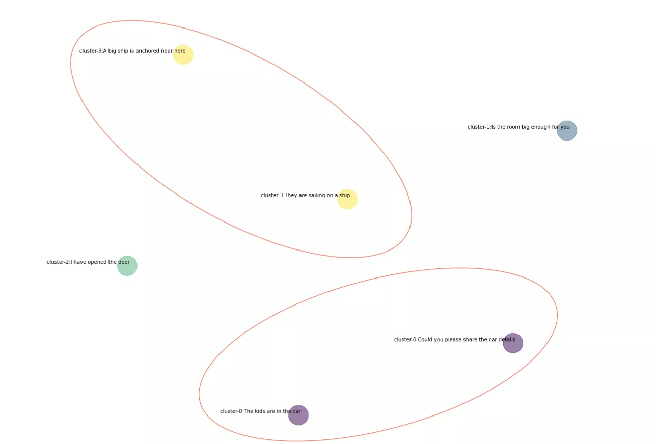
We can see that even though the sentences look apart on the 2D plane, they are basically part of the same cluster and are indeed very similar sentences.
That’s all for this post. Hope it was helpful.